Reading Data
Direct entry, Data frames
Ben Dickins
Inputting Data
R allows users to input data using a wide range methods. - Directly by typing the data into R (using scan()) - Reading external files: txt, csv, SAS, SPSS, Excel.
I encourage you to learn different methods, but we will cover a common and robust use case: handling csv files. For more information follow this advice.
Inputting Data
Direct Method
You can directly input data points one by one using scan()
Do it yourself:
This is called a base function.
Inputting Data
External Files
External files come in various formats and a number of convenience functions are available:
- read.table()
- read.csv()
- read.delim()
Before we need to find out our working directory:\
Do it yourself:
Inputting Data
Setting Paths
You can use dir() to find what is in each directory and setwd() to change to a new working directory.
Do it yourself: We are going to change working directory to the revanent-master folder we put in the OneDrive folder earlier:
Do it yourself:
Read the simple.txt data set and store it in a data frame called easy:
Let us look at the first 6 lines of the data:
There’s also an RStudio command (note uppercase letter) for looking at a data frame:
Plotting
Now plot the data!
Inputting Data
Comma Separated
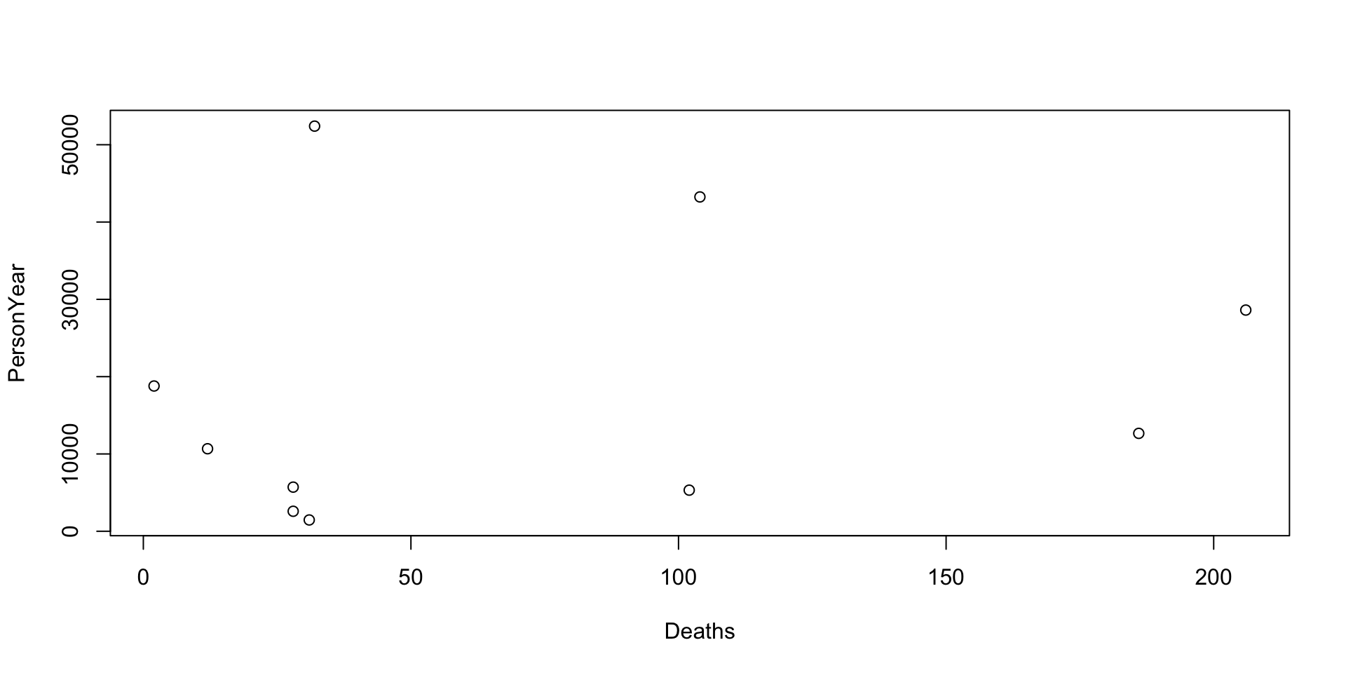
Do it yourself: Read the smoking.csv data set and store it in a data frame called smoking:
Let’s look at the data too:
Data Frames
- A data frame is a list of variables, each of the same length but not necessarily of the same type.
- The top line of the table, called the header, contains the column names.
- Each horizontal line afterward denotes a data row, which begins with the name of the row, and then followed by the actual data.
Built-in Data Frames
- We can also call built-in data frames in
Rfor our tutorials. - This can be done by using the
data()command. - For example, here is a built-in data frame in
R, calledmtcars.
Do it yourself:
Call the R built-in data set mtcars as follows:
Let us look at the first 6 lines of the data:
                   mpg cyl disp  hp drat    wt  qsec vs am gear carb
Mazda RX4         21.0   6  160 110 3.90 2.620 16.46  0  1    4    4
Mazda RX4 Wag     21.0   6  160 110 3.90 2.875 17.02  0  1    4    4
Datsun 710        22.8   4  108  93 3.85 2.320 18.61  1  1    4    1
Hornet 4 Drive    21.4   6  258 110 3.08 3.215 19.44  1  0    3    1
Hornet Sportabout 18.7   8  360 175 3.15 3.440 17.02  0  0    3    2
Valiant           18.1   6  225 105 2.76 3.460 20.22  1  0    3    1
Find out more about it:
The Environment
Do it yourself: See all the objects and data in your environment:
Or you can see it in the top right corner of RStudio (Environment tab).